Before reading, you can try out my interactive visualization tool for a primer on what I’ll discuss below.

At their core, neural networks are functions. They take some input, perform a series of computations, and produce an output. Though most networks operate in the realm of vectors and matrices, it can be a useful exercise to see them without the extra barrier of linear algebra. For this purposes of this explanation, we will only cover single variable functions, but the principles we will see can be extended into any number of dimensions.

The Forward Pass

Before we reach the backwards propagation of gradients, we will observe the forward propagation of values. The forward pass provides a reasonable basis for understanding how functions can be represented as the result of other functions combined. Finally, we can represent these functions as a computation graph—an idea which will be useful when we arrive at the backward pass of the function.

Function Composition

We begin with the most basic function, mapping the entire range of inputs to a single number.

$f(x) = 1$

Simple, right? Let’s try to incorporate $x$ into the mix by creating the identity function—any $x$ in will be the same $x$ out.

$g(x) = x$

The power comes when we can compose the functions using different operations, building a new function from the existing ones. By composing functions together, we can evaluate the individual functions before we evaluate the parent.

$h(x) = f(x) + g(x) = 1 + x$

Likewise, we can feed the output of one function as the input of another, increasing the complexity of the overall function while retaining its individual parts.

$f(x) = 7x + 3$

$g(x) = x^2$

$h(x) = g(f(x)) = (7x + 3)^2$

Intuitively, a human would first calculate the value of $7x+3$ before squaring the result. This staged ordering creates a hierarchy of functions that our algorithms can harness.

We see this type of hierarchy building when we build models in any machine learning library. What TensorFlow calls a “model” is just a series of computations composed into a single function.

model = tf.keras.Sequential()

model.add(Dense(512))
model.add(Dense(512))
...
model.add(Dense(32))
model.add(Dense(10))

# Outputs the result of sequentially feeding X through the Dense layers
y = model.predict(X)

Every time we call model.add(), we are adding to the hierarchy that defines our neural network. In machine learning, composed functions $h(x)$ defined earlier are less like $f(x)+g(x)$ and more like

$h(x) = f_5(f_4(f_3(f_2(f_1(x))))).$

Each $f_n$ is a layer in the network which produces an output by using the previous layer as input.

Building a Computation Graph

We can visualize a composed function’s structure as a tree, each layer representing a different stage of the operation. In fact, most programming languages use a parse tree to store and evaluate expressions in code. This representation gives us the ability to view a function in terms of its component parts, recursing down the levels until we find the constants and variables at the very bottom.

For example, take the function $f(x)$ given below.

$f(x) = \frac{1}{1+e^{-x}}$

In machine learning, this is a function called the sigmoid, often written as $\sigma(x)$. Let’s see how we could break the sigmoid into a computation tree.

Notice how all four leaf nodes are either a constant or a variable. These are the most elementary parts of any composite function. We can even give the intermediate functions letter names to highlight how each node is built from its children.

The equations for our new tree would be

$a=e, b=-x,f=1,d=1$

$c = a^b$

$e = c+d$

$g = \frac{f}{e}$

The Backward Pass

Up until this point, viewing functions as hierarchies seems to add unnecessary abstractions on a relatively simple topic. However, now that we have observed how to compute the “forward pass” of a computation graph, we can compute the reverse using an algorithm called backpropagation.

Gradient Descent

In machine learning, the end goal is to minimize error on a loss function, and modern software achieves this goal through an algorithm called gradient descent. Though I will not attempt to explain the entirety of gradient descent here, a basic understanding of how it works is essential for understanding backpropagation.

Loss functions measure how much the outputs of a model, the neural network, deviate from the labels in a dataset. Tuning the parameters of the model will either increase or decrease that loss, and the goal is to find the set of parameters that will give us the minimum loss. Through gradient descent, we try to estimate which direction we should tune our model in order to achieve the optimal settings.

Imagine we have a loss function $L$ that measures the performance of a model with only one parameter, $p$. The graph of $L$ could look something like this graph:

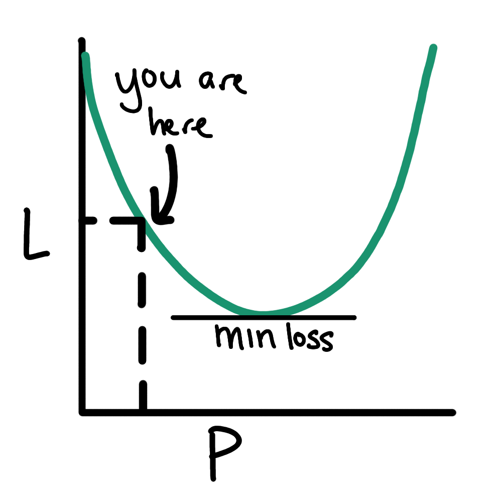
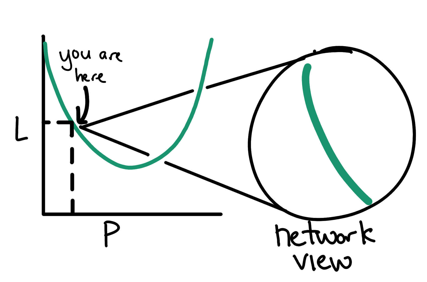
From this zoomed out perspective, the valley in the curve (where loss is the lowest) is obvious. However, when we train a model, this view is significantly smaller, giving us only information about how the loss curve looks near the current value of $p$.

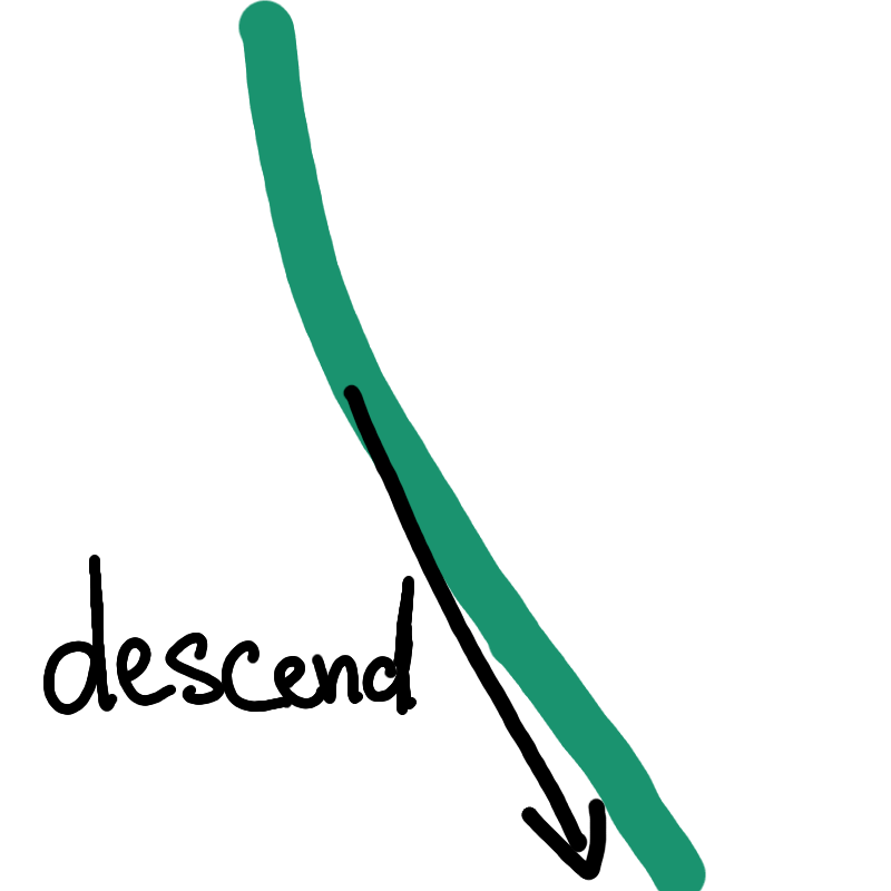
Intuitively, we should follow the direction that has the steepest slope downwards to find the minimum. In mathematical terms, we want to look at the gradient of $L$ and take a small step in the direction down that gradient.

Backpropagation is the tool that helps a model find that gradient estimate so that we know which direction to move in.

Backpropagation

The gradient is a collection of slope calculations called the partial derivatives. Both partial derivatives and gradients answer a question that is fundamental to our purpose: how does a small change in a variable $x$ respectively change the output function $f(x)$. In machine learning, we want to observe how changing $x$ will change the loss.

Before we begin, let us revisit some of the basic rules of calculus that are crucial to understanding backpropagation. When computing partial derivatves, we consider other variables of the functions constants, so $c$ represents any constant or variable other than $x$.

$\frac{\partial}{\partial x} (c)=0$

$\frac{\partial}{\partial x} (cx)=c$

$\frac{\partial}{\partial x} (x^n)=nx^{n-1}$

$\frac{\partial}{\partial x} (a^x)=a^x \ln a$

$\frac{\partial}{\partial x} (\log_a x)=\frac{1}{x \ln a}$

$\frac{\partial}{\partial x} (f+g)=\frac{\partial f}{\partial x} + \frac{\partial g}{\partial x}$

$\frac{\partial}{\partial x} (fg)=f\frac{\partial g}{\partial x} + g\frac{\partial f}{\partial x}$

$\ldots$

There are many more rules, but these basics encompass a large portion of what functions you might see in machine learning applications. However, using only these rules, our function vocabulary is significantly limited. We can only take partial derivatives for simple functions like $5x$ or $3^x + 2x$ if we are clever. The essential property for achieving infinitely complex functions is a rule most calculus classes group with the rest.

$\frac{\partial}{\partial x} f(g(x)) = \frac{\partial f}{\partial g} \frac{\partial g}{\partial x}$

The chain rule enables us to unravel the composed functions we discussed earlier—giving us the ability to compute arbitrarily complex partial derivatives and gradients. Using the computation graph we constructed earlier, we can move backwards from the final result to find individual derivatives for variables. This backwards computation of the derivative using the chain rule is what gives backpropagation its name. We use the $\frac{\partial f}{\partial g}$ and propagate that partial derivative backwards into the children of $g$ .

As a simple example, consider the following function and its corresponding computation graph.

$g(x)=(4x+1)^2$

As earlier, we assign the intermediate computations letter names to use in calculation. Let’s find $\frac{\partial g}{\partial x}$, the slope of $g(x)$, when $x=1$. First, let’s compute the forward pass of the function, labelling the intermediate values of each node until we reach $g(1)=25$.

Starting from the top, let us find the partial derivatives of the tree on the path down to $x$. As we traverse down the tree, it only makes sense to take the partial derivatives with respect to the branches that $x$ is a part of.

$g=e^f \rightarrow \frac{\partial g}{\partial e}=fe^{f-1}$

Since $e$ is a direct child of g, the chain rule is not necessary here. Knowing the values of $f$ and $e$ from the forward pass, we can find a numerical value for the partial derivative.

$\frac{\partial g}{\partial e}=2 \times 5^1=10$

The next node in the path is $c$, a direct child of the previous node $e$. To find the “local” partial derivative, $\frac{\partial e}{\partial c}$ we use the addition rule. $\frac{\partial c}{\partial d}$ is 0 since a small change in $d$ makes no change in $c$

$e = d + c$

$\frac{\partial e}{\partial c} = \frac{\partial d}{\partial c} + \frac{\partial c}{\partial c} = 0 + 1 = 1$

To find the desired value of $\frac{\partial g}{\partial c}$, we can finally employ the chain rule.

$\frac{\partial g}{\partial c} = \frac{\partial g}{\partial e}\frac{\partial e}{\partial c} = 10 \times 1 = 10$

Finally, we arrive at node $b$, the node containing $x$. The process for finding this derivative is identical to the previous ones.

$c = ab$

$\frac{\partial c}{\partial b} = a = 4$

$\frac{\partial g}{\partial b} = \frac{\partial g}{\partial c}\frac{\partial c}{\partial b} = 10 \times 4 = 40$

We’ve arrived at the end of the path to $x$, giving us the final value of $\frac{\partial g}{\partial x} = 40$.

I encourage you to revisit my visualization tool and play around with various functions, tracing the path of the gradients down to your original variables. You might even want to try (4*x+1)^2 and see how the gradients change as $x$ changes.

This simple algorithm for calculating partial derivatives on a computation graph is very similar to the way neural networks are trained in libraries like Tensorflow. A firm understanding on how the libraries work allows you to expand your capabilities beyond the prepackaged layers they provide. More importantly, it allows you to gain insight on the algorithms used every day to train computers on any amount of data.

The task remains constant—minimize error on a loss function.

Additional Resources

This post was inspired by the insightful explanations of backpropagation linked below.

Stanford CS231n - Backpropagation, Intuitions

3Blue1Brown - What is backpropagation really doing?

Welch Labs - Neural Networks Demystified - Backpropagation